A model that predicts nothing scores 89.83% accuracy
Given a comment, predict all applicable policy labels — toxic, severe_toxic, obscene,
threat, insult, identity_hate — not just the most likely one. Fine-tuned DistilBERT on the
Kaggle Jigsaw Toxic Comment Classification data (159,571 Wikipedia comments).
The project is organised around one claim: accuracy is the wrong metric here. A model that
predicts nothing at all scores 89.83% exact-match accuracy and 99.70% on threat on
this data, at a macro-F1 of exactly 0.0. So the work isn’t squeezing the model — it’s
choosing the right metric, calibrating a threshold per label, and doing real error analysis.
- Code: Srijan-Ratrey/Multilabel-content-classification
- Model: srijanratrey/distilbert-jigsaw-multilabel
- Build brief: tech-spec.md
Results
Held-out test split, n=23,936. Macro-F1 is the headline; “tuned” means per-label thresholds calibrated on validation and applied unchanged to test.
| model | macro-F1 @0.5 | macro-F1 tuned | micro-F1 tuned |
|---|---|---|---|
| all-zeros control | 0.0000 | — | — |
| TF-IDF + OvR logistic regression, unweighted | 0.4692 | 0.5964 | 0.7249 |
| TF-IDF + OvR logistic regression, balanced | 0.5412 | 0.6112 | 0.7235 |
| DistilBERT | 0.6626 | 0.6836 | 0.7875 |
Per-label, for the final model (macro-AP 0.7359, Hamming loss 0.0158):
| label | threshold | precision | recall | F1 | AP | test positives |
|---|---|---|---|---|---|---|
toxic | 0.55 | 0.847 | 0.832 | 0.839 | 0.921 | 2,295 |
obscene | 0.65 | 0.832 | 0.826 | 0.829 | 0.910 | 1,268 |
insult | 0.50 | 0.733 | 0.787 | 0.759 | 0.832 | 1,181 |
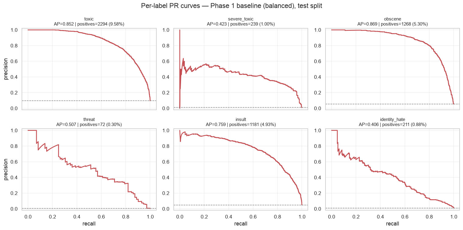
identity_hate | 0.50 | 0.667 | 0.535 | 0.594 | 0.641 | 213 |
severe_toxic | 0.25 | 0.441 | 0.697 | 0.540 | 0.573 | 241 |
threat | 0.20 | 0.456 | 0.662 | 0.540 | 0.538 | 71 |
Key findings
Accuracy is disqualified. The all-zeros control scores 89.83% exact-match and 96.33% mean
per-label accuracy at macro-F1 0.0. Accuracy rewards predicting the majority class, and here
89.8% of comments carry no label at all. It appears in this repo only inside each result’s
all_zeros_baseline block, as a control.
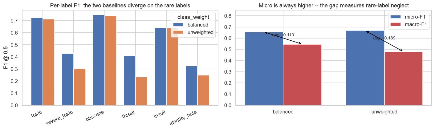
Micro-F1 would have selected the worse model. The unweighted baseline beats the balanced one
on micro-F1 (0.6716 vs 0.6591) while losing badly on macro-F1 (0.4692 vs 0.5412). It buys that
micro-F1 by being precise on frequent labels and nearly silent on rare ones — at threshold 0.5
it predicts threat just 9 times against 71 true positives. Micro pools every decision, so
toxic’s 2,295 positives outvote threat’s 71 by ~32:1; macro weights the six labels equally.
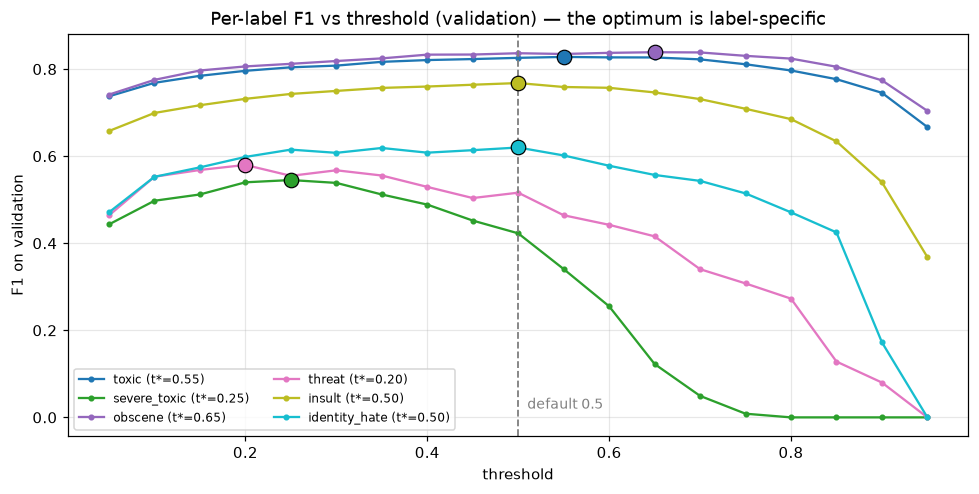
Thresholds are worth more than they look. Moving off 0.5 gains +0.070 macro-F1 on the
baseline (+12.9%) and +0.021 on the transformer, with no retraining. The gain is concentrated where
it matters: on the transformer, severe_toxic +0.085 and threat +0.040. The gain shrinks as
the model improves, which is the honest read — a better-calibrated model has less to recover at
the operating point.
An undertrained model silently ignored its rarest label. A first training run (lr 2e-5)
scored macro-F1 0.5671 and predicted threat zero times — F1 0.000 with AP 0.257. Raising
the learning rate to 3e-5 took it to 0.6626 with threat F1 0.500. Both runs reached the same
3,492 optimizer steps, so the entire difference was the learning rate, not training length.
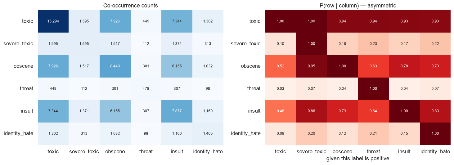
One-vs-Rest cannot represent the label structure. Every label is close to a subset of
toxic: P(toxic | severe_toxic) = 1.000 exactly, and P(toxic | ·) ≥ 0.927 for all five others.
obscene↔insult overlap 0.781/0.728. Six independent classifiers have no mechanism for any of
this — the motivation for the classifier-chains comparison in Phase 6.
Design decisions worth knowing
Sigmoid + BCE, not softmax. The output layer is six independent sigmoids trained with
BCEWithLogitsLoss. Softmax normalises across labels, forcing them to compete and sum to 1 —
it cannot represent a comment that is toxic and obscene and insulting, nor the all-zero case
that covers 89.8% of this dataset.
The Jigsaw -1 trap. test_labels.csv has 153,164 rows, but 89,186 carry -1 in every
label — withheld from the original competition’s scoring. -1 means unknown, not negative;
only 63,978 rows are scoreable. Evaluating against the unfiltered file treats 89,186 unknowns as
negatives and produces meaningless metrics. The filter lives once in
load_kaggle_test
behind assertions. The project’s own train/val/test all come from train.csv, so the main
pipeline never touches it.
Splits are frozen and stratified on the label combination. 70/15/15, persisted to
data/processed/splits.npz. Stratifying on the exact 6-label combination is finer than
per-label stratification and needs only scikit-learn, so the CLI, the notebook, and a Kaggle run
produce identical splits. threat lands at 335 train / 72 val / 71 test positives.
Thresholds are tuned on validation, never on test. The 19-point grid is deliberately coarse:
with 72 validation positives for threat, a finer grid fits noise.
Padding strategy was worth ~3x. Median comment is 52 tokens against a 256 limit. Dynamic padding alone barely helps — random batches still pad to 250.8 of 256, because a batch of 32 almost always catches one long comment. With length-grouped batching the mean batch width drops to ~81, which is what takes the run from ~2h25m to ~45min on an M4.
Limitations
- English only, and it fails silently elsewhere. The model scores a Hinglish death threat
(
"tujhe jaan se maar dunga") atthreat=0.000and fires no labels on any Hindi or Hinglish input. This is not degradation, it is silent failure — the worst error mode for a safety classifier.distilbert-base-uncasedshreds Devanagari into meaningless single characters and maps Hinglish onto unrelated English word-pieces. Do not deploy this on non-English content. - Rare labels are weak. F1 ≈ 0.54 on
threatandsevere_toxic;identity_haterecall is 0.535, so it misses about half of them. threat’s threshold rests on 72 validation positives, so its tuned score is a noisy estimate — its validation-to-test F1 gap is −0.040.- Trained on 2018 English Wikipedia talk-page comments. Other platforms, domains and eras will degrade, likely a lot.
- Inputs are truncated at 256 tokens, which cuts 6.93% of comments (17.44% of all tokens).
- A demo, not a moderation system. Don’t make consequential decisions about people with it.
Running it
Python 3.11+ required (developed on 3.12).
git clone https://github.com/Srijan-Ratrey/Multilabel-content-classification.git
cd Multilabel-content-classification
python -m venv .venv && source .venv/bin/activate     # or: uv venv --python 3.12 .venv
pip install -r requirements.txt
Data. Download the Kaggle
Jigsaw Toxic Comment Classification Challenge
files and place them in data/raw/ (gitignored, ~140MB). Only train.csv is needed for the
pipeline. Then build the label matrix and freeze the splits:
python -m src.dataClassify your own text (needs a trained model):
python -m src.predict --interactive
python -m src.predict "you are an idiot"
python app.py                      # Gradio UI at http://127.0.0.1:7860
Training: use the notebook
notebooks/train_model.ipynb
is self-contained — no src/ imports — so it runs on Kaggle or Colab as well as locally. It
finds train.csv automatically (including under /kaggle/input), adapts to whichever
transformers version is installed, trains, evaluates, calibrates thresholds, and writes every
artifact the analysis reads.
Set QUICK_TEST = True for a ~2 minute smoke run first. Full run: ~21 min on a Kaggle T4,
~45 min on an Apple M4 (MPS).
Or the CLI, phase by phase
python -m src.data                                   # splits -> data/processed/splits.npz
python -m src.baseline --class-weight balanced       # Phase 1
python -m src.baseline --class-weight none           #   the unweighted contrast
python -m src.evaluate --probs models/probs/baseline_test.npy --split test \
    --out results/phase2_baseline_test.json --plots results/pr_baseline.png
python -m src.transformer --token-stats              # measure truncation cost first
python -m src.transformer                            # Phase 3
python -m src.thresholds --model transformer         # Phase 4.1
Every command writes its metrics to results/*.json and its plots to results/*.png, so
phases stay comparable.
Reproducibility
SEED = 42 is set for random, numpy and torch from one place
(src/config.py)
and logged on every entry point. Splits are frozen on disk and reused by every phase. Every
metric is written to results/ as JSON so phases can be compared rather than re-derived.
Dataset: Kaggle Jigsaw Toxic Comment Classification Challenge (CC0, Wikipedia comments).